Your body is unique. That is exactly what we solve for.

In 1973 S. S. Wilson plotted the cost of transport — energy spent per gram of body weight per kilometre — for everything that moves, from a fruit fly to a jet transport. A human walking is unremarkable, sitting mid-field with the dogs and the horses.

Put the same human on a bicycle and they drop off the bottom of the chart. Not marginally: roughly a fifth of the energy of walking, and better than every animal and every machine on the plot.

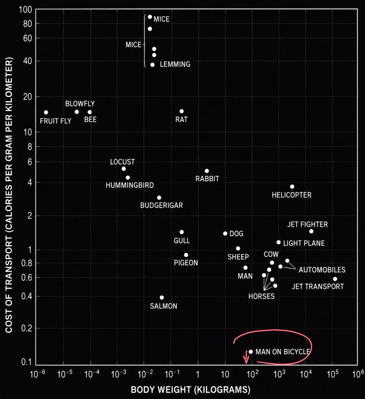
The bicycle is not the inefficiency — it is arguably the most efficient machine ever built for moving a body.

The red arrow points straight down, because on this chart down means less energy spent to cover the same kilometre. Driving that point lower is what we optimise for.

And once the machine is already this good, lower no longer comes from equipment. It comes from the rider and the air around them — from what shape you present to the wind. That is the part nobody has measured for you.

Your two full-body images are read by an AI model that projects you into a parametric shape space — on the order of 100 parametersdescribing segment lengths, girths, torso depth and width, limb proportion, and the postural defaults your skeleton sits in.

The frontal view constrains your width and the side view constrains your depth. Two orthogonal silhouettes are enough to pin down a body in three dimensions once the model already knows what human proportions look like — that prior is what makes two photographs sufficient rather than a full photogrammetry rig.

Everything is dimensionless until your height is applied. That single scalar sets the scale of the whole model, and every area and length downstream inherits it.

The on-bike photographs solve a different problem: not what shape are you but what configuration are you in. Hip angle, torso inclination, shoulder position, elbow flexion, head carriage, hand location.

The body from step one is articulated into that configuration. Each position you submit becomes its own posed geometry — the same underlying body, presenting a different surface to the oncoming air. That distinction matters: your shape is constant across the comparison, so any difference the solver reports comes from posture alone.

CFD — Computational Fluid Dynamics replaces a physical wind tunnel with a numerical one. The behaviour of air is described by the Navier–Stokes equations: conservation of mass and of momentum, written for a continuous fluid.

There is no general closed-form solution to these. So instead of solving them analytically, you chop the air around the body into millions of small cells — the mesh — and solve a discretised version of the equations in every cell, iterating until the residuals fall and the flow field stops changing. That is convergence, and it is the point at which the answer is worth reading.

At riding speeds the flow is fully turbulent, and resolving every eddy directly is computationally out of reach for a service at this price. The practical approach is to solve the averaged flow and model the turbulence statistically, which is the standard trade in applied external aerodynamics: you give up the instant-by- instant detail and keep the forces, which is what a rider actually wants.

Right at your skin, air is stationary — the no-slip condition. A few millimetres out, it is moving at full speed. That gradient is the boundary layer, and almost everything interesting happens inside it.

Over the front of your body the pressure falls and the boundary layer stays attached. Past the widest point the pressure starts rising again — an adverse pressure gradient — and the slow-moving air nearest the surface no longer has the momentum to push against it. At some point it stops, reverses, and separates from the surface.

Behind the separation line sits a turbulent, low-pressure wake. The high pressure on your chest and the low pressure in that wake is a net force pulling you backwards — this is pressure drag, and on a cyclist it dominates the skin-friction component by a wide margin.

Where separation happens depends on your surface curvature, your posture, and your speed. Change your seat position and you change the curve the flow has to negotiate. This is why two positions with near-identical frontal area can measure differently, and why the ranking can shift between 30 km/h and 45 km/h — the separation point moves.

CdA is drag area, in square metres — the drag coefficient Cd multiplied by frontal area A. Cd captures how slippery the shape is independent of size; A captures how much of you the air has to get around. They are reported together because drag depends on the product, and separating them invites you to optimise the wrong one.

A rider with CdA ≈ 0.30 m² at 40 km/h in 25 °C air is spending roughly 240 W on air resistance alone. Because the relationship is cubic, the same CdA reduction is worth (45/35)³ ≈ 2.1× as many watts at 45 km/h as at 35. Aerodynamics rewards the fast disproportionately, which is precisely why it is worth measuring rather than guessing.

The Reynolds number is the ratio of inertial to viscous forces, and it decides what the flow regime looks like.

A cyclist at 40 km/h with L ≈ 0.4 m sits around Re ≈ 3 × 10⁵. That is squarely in the range where boundary-layer behaviour is sensitive to both geometry and speed — not so slow that viscosity dominates, not so fast that the separation point is pinned. It is also why a result is quoted across a speed range rather than as a single figure.

Every simulation runs at the same condition, so that the only variable between two of your positions is the position.

Density matters more than it sounds. Air at 25 °C is about 3.3% less dense than at 15 °C, and drag scales linearly with density — so an unfixed temperature would smear a few percent of noise across every comparison, which is the same order as the effect being measured.

Only the rider goes into the domain. Including the bicycle would add spokes, tubes, bottles and drivetrain — geometry with small features that force a much finer mesh, a much larger cell count, and a solve time that scales with it. The cost of a simulation would rise sharply.

And it would buy very little of what you came for. For the same rider on the same bike in two positions, the bicycle contributes near-identical drag in both runs. In a difference it very largely cancels. What changes between your positions is you, so that is where the compute goes.

The honest consequence: WattCut reports the delta your position makes, not the absolute CdA of the rider-plus-bicycle system. If you want an absolute number to compare against a published figure, this is not that measurement.

A simulation built from two photographs is an estimate with a real error bar. Photogrammetric reconstruction, a statistical body prior, a modelled turbulence closure and an absent bicycle each contribute uncertainty, and none of them is zero. It will not match a physical tunnel and WattCut does not claim it does.

What it is built to do is rank your own positions against each other under conditions held identical, where the shared error sources largely cancel and the difference is the signal. Treat the output as information, not instruction — the fastest position is only worth anything if you can breathe in it, see out of it, handle the bike in it and still produce power in it.